Inference after Hierarchical and k-means clustering

Introduction

This vignette demonstrates how to use test.clusters.hc() and test.clusters.km() functions from the PCIdep package to perform post-clustering inference on hierarchical agglomerative clustering (HAC) and k-means clustering results. We’ll use the Palmer penguins dataset as an example.

This vignette is an adaptation of Lucy L. Gao’s great tutorial.

The Palmer Penguins Data

The Palmer Penguins dataset contains measurements of penguin species collected from the Palmer Station in Antarctica. It includes data on body measurements (bill length, flipper length, body mass) and other characteristics for three penguin species: Adelie, Chinstrap, and Gentoo. This dataset is a useful toy example for demonstrating clustering and classification techniques.

Reference: Horst, A. M., Hill, A. P., & Gorman, K. B. (2020). palmerpenguins: Palmer Archipelago (Antarctica) penguin data. Retrieved from https://github.com/allisonhorst/palmerpenguins

library(palmerpenguins)
#> 
#> Attaching package: 'palmerpenguins'
#> The following objects are masked from 'package:datasets':
#> 
#>     penguins, penguins_raw
data(penguins)
head(penguins)
#> # A tibble: 6 × 8
#>   species island    bill_length_mm bill_depth_mm flipper_length_mm body_mass_g
#>   <fct>   <fct>              <dbl>         <dbl>             <int>       <int>
#> 1 Adelie  Torgersen           39.1          18.7               181        3750
#> 2 Adelie  Torgersen           39.5          17.4               186        3800
#> 3 Adelie  Torgersen           40.3          18                 195        3250
#> 4 Adelie  Torgersen           NA            NA                  NA          NA
#> 5 Adelie  Torgersen           36.7          19.3               193        3450
#> 6 Adelie  Torgersen           39.3          20.6               190        3650
#> # ℹ 2 more variables: sex <fct>, year <int>

We are interested in classifying individuals based on bill and flipper length, using species as the ground truth for evaluating the clustering results.

data_penguins <- penguins[penguins$sex == "female", c("bill_length_mm", "flipper_length_mm", "species")]
data_penguins <- na.omit(data_penguins)

The scatter plot below illustrates the distribution of female penguins in the bill length vs. flipper length space, colored by species. It provides an initial visual assessment of how well these two measurements separate the three penguin species, motivating the use of clustering.

library(ggplot2)
ggplot(data_penguins, aes(x = bill_length_mm, y = flipper_length_mm, color = species)) +
  geom_point() +
  theme_bw() +
  labs(title = "Female Penguins: Bill Length vs Flipper Length")+
  labs(x = "Bill Length (mm)", y = "Flipper Length (mm)", color = "Species")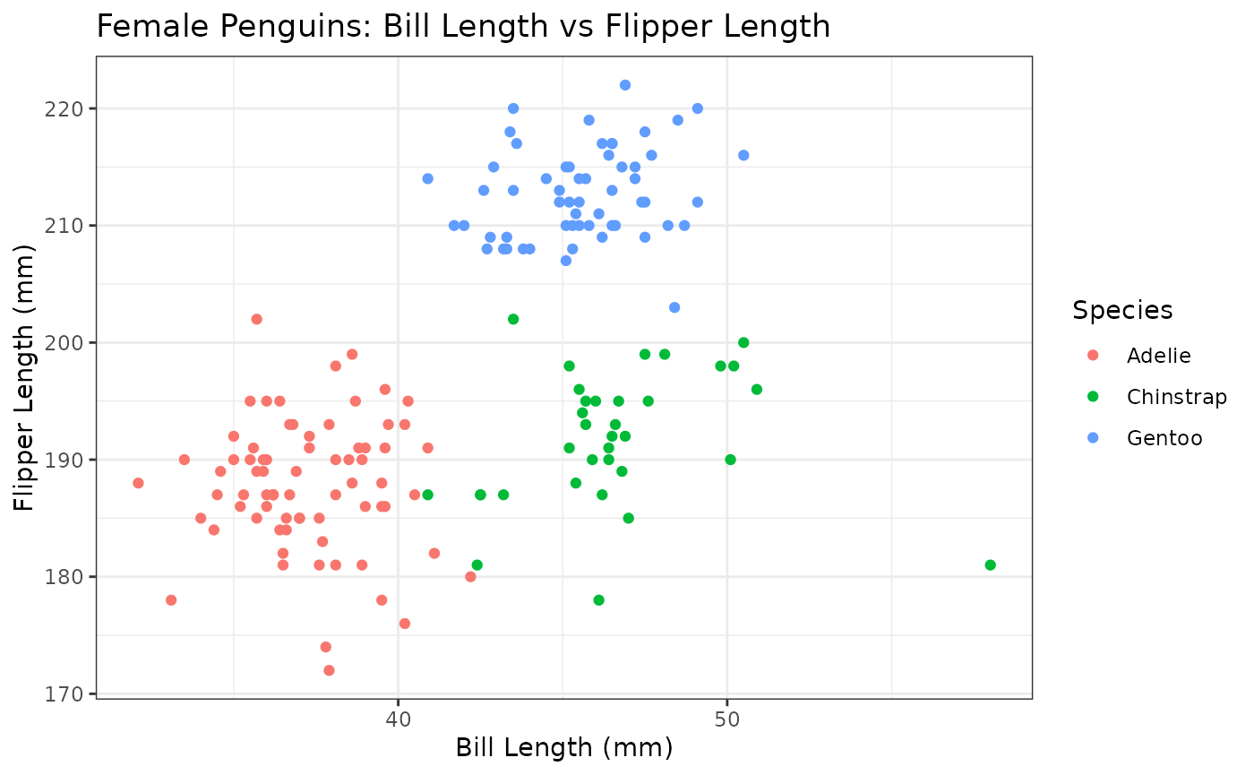

Inference after Hierarchical Clustering with `test.clusters.hc()`

Performing HAC

Hierarchical Agglomerative Clustering (HAC) starts with each observation as its own cluster and iteratively merges the closest clusters according to a linkage criterion. Here, we use single linkage (single). After building the dendrogram, we cut it at K=5 to obtain five groups.

# Perform hierarchical clustering
X <- data_penguins[, c("bill_length_mm", "flipper_length_mm")] # Clustering based on bill length and flipper length
hc_result <- hclust(dist(X), method = "ward.D") # HAC with Ward linkage

# Cut the dendrogram to get cluster assignments
num_clusters <- 5
hc_clusters <- cutree(hc_result, k = num_clusters)

# Scatter plot: color by species and use markers for HAC clusters
ggplot(data_penguins, aes(
  x = bill_length_mm,
  y = flipper_length_mm,
  color = species,
  shape = factor(hc_clusters)
)) +
  geom_point(size = 2.5, alpha = 0.85) +
  theme_bw() +
  labs(
    title = "Female Penguins: Species colors and HAC cluster markers",
    x = "Bill Length (mm)",
    y = "Flipper Length (mm)",
    color = "Species",
    shape = "HAC cluster"
  )

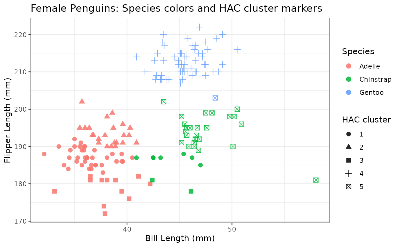
The previous plot shows that some species were correctly classified into a single cluster, like Gentoo, but we also have different species classified into the same cluster (cluster 1) and two clusters containing individuals from the same species (2 and 3). This motivates the use of post-clustering inference to assess whether the retrieved clusters correspond to the known ground truth.

Covariance estimation is needed for post-clustering inference

The data model in PCIdep allows for an arbitrary covariance matrix describing dependency between features. Since the true covariance matrix \boldsymbol{\Sigma} is unknown, we estimate it while maintaining statistical guarantees. There are two options to estimate \boldsymbol{\Sigma} in PCIdep, detailed below. These hold for all clustering algorithms implemented in the package, including HAC (test.clusters.hc()), k-means (test.clusters.km()) and any custom clustering algorithm (test.clusters.MC()).

1. Sample splitting

Data can be split into two sub-samples. One sub-sample is used to estimate \boldsymbol{\Sigma} and the other is used for clustering and inference. This approach is valid under the assumption of independence between observations. To implement this, set sample_split = TRUE in the testing function. The user can also specify the number of observations to use for covariance estimation via the nY parameter, which defaults to half of the total sample size.

⚠ Important
If sample splitting is performed internally (setting sample_split = TRUE), clustering (and testing) will be performed on a random subset of X. Consequently, any further analysis or representation of the retrieved clusters should be performed on such data subset. To obtain the data subset used for clustering and inference, set return_X_clus = TRUE when calling the function. This will include the data matrix used for clustering in the returned list under the name X_clus. If preferred, the user can also perform sample splitting prior to calling the function, and provide the covariance estimation sample via the Y parameter (see next section). In this case, clustering and inference will be performed on the full data matrix X.

2. Provide an independent sample

If an independent sample is available, it can be provided directly to the testing function via the Y parameter. Then, Y will be used to estimate \boldsymbol{\Sigma} while the full sample X is used for clustering and inference. When an i.i.d. sample is available, this approach is more powerful than sample splitting since it uses the full data for clustering and inference, while still providing valid covariance estimation.

💡 Dependent observations
This functionality allows introducing an i.i.d. sample for estimation when observations are not independent, that is, whose covariance structure is encoded via a known matrix \mathbf{U}\neq\mathbb{I}_n. A matrix \mathbf{U} of size n_Y \times n_Y, where n_Y is the number of observations in the i.i.d. copy, must be provided via the UY parameter. Alternatively, its inverse (precision matrix) can be supplied via the precUY parameter. If neither of UY or precUY is provided, the function will assume independence between observations in the i.i.d. copy and set UY to the identity matrix.

Testing cluster differences with `test.clusters.hc()`

Now we are interested in assessing whether the difference between the retrieved clusters are statistically significant. To do so, we use the test.clusters.hc() function.

📝 Note
The test.clusters.hc() function does not require the clustering to be performed beforehand. It performs the hierarchical clustering automatically given a linkage method and a number of clusters, so the previous code was only illustrative. However, if the user prefers to perform clustering beforehand, they can provide a stats::hclust() or fastcluster::hclust() object via the hcl parameter, as well as the squared distance matrix via the dismat parameter. In this case, the function will not perform clustering and will directly test the provided clusters. This can be useful when multiple cluster pairs from the same partition or dendrogram are to be tested.

Here, if we assume that the dependence between flipper and bill length is the same across sexes, we can use the male penguins data to estimate \boldsymbol{\Sigma}:

Y <- penguins[penguins$sex == "male", c("bill_length_mm", "flipper_length_mm")]
Y <- na.omit(Y) # i.i.d. sample for covariance estimation

Then, we run test.clusters.hc(), setting the following parameters:

X: data matrix used for clustering and inference.
Y: independent sample used for covariance estimation.
NC: number of clusters to retrieve from the dendrogram.
clusters: pair of cluster labels to compare (e.g., c(1, 2)).
linkage: HAC linkage method (here, "ward.D").
U: covariance matrix of observation-level dependence. Here observations are assumed independent, so U is set to the identity matrix, which is the default.

For details on the parameters and their usage, please refer to the test.clusters.hc documentation.

# Test the HAC clusters

# Difference between clusters 4 and 2 (different species)
hc_test_42 <- PCIdep::test.clusters.hc(X=X, Y=Y, NC = 5, clusters = c(4, 2), linkage = "ward.D")
#> U is not provided: observations are considered independent with unit variance.
#> Sigma not provided: plugging an over-estimate.
hc_test_42$pvalue 
#> [1] 0.0001055019

# Difference between clusters 2 and 3 (same species)
hc_test_23 <- PCIdep::test.clusters.hc(X=X, Y=Y, NC = 5, clusters = c(2, 3), linkage = "ward.D")
#> U is not provided: observations are considered independent with unit variance.
#> Sigma not provided: plugging an over-estimate.
hc_test_23$pvalue
#> [1] 0.8907002

The results correspond to the expected behavior: the difference between clusters 4 and 2 is significant (as they contain different species), while the difference between clusters 2 and 3 is not significant (as they contain individuals from the same species).

k-means Clustering with `test.clusters.km()`

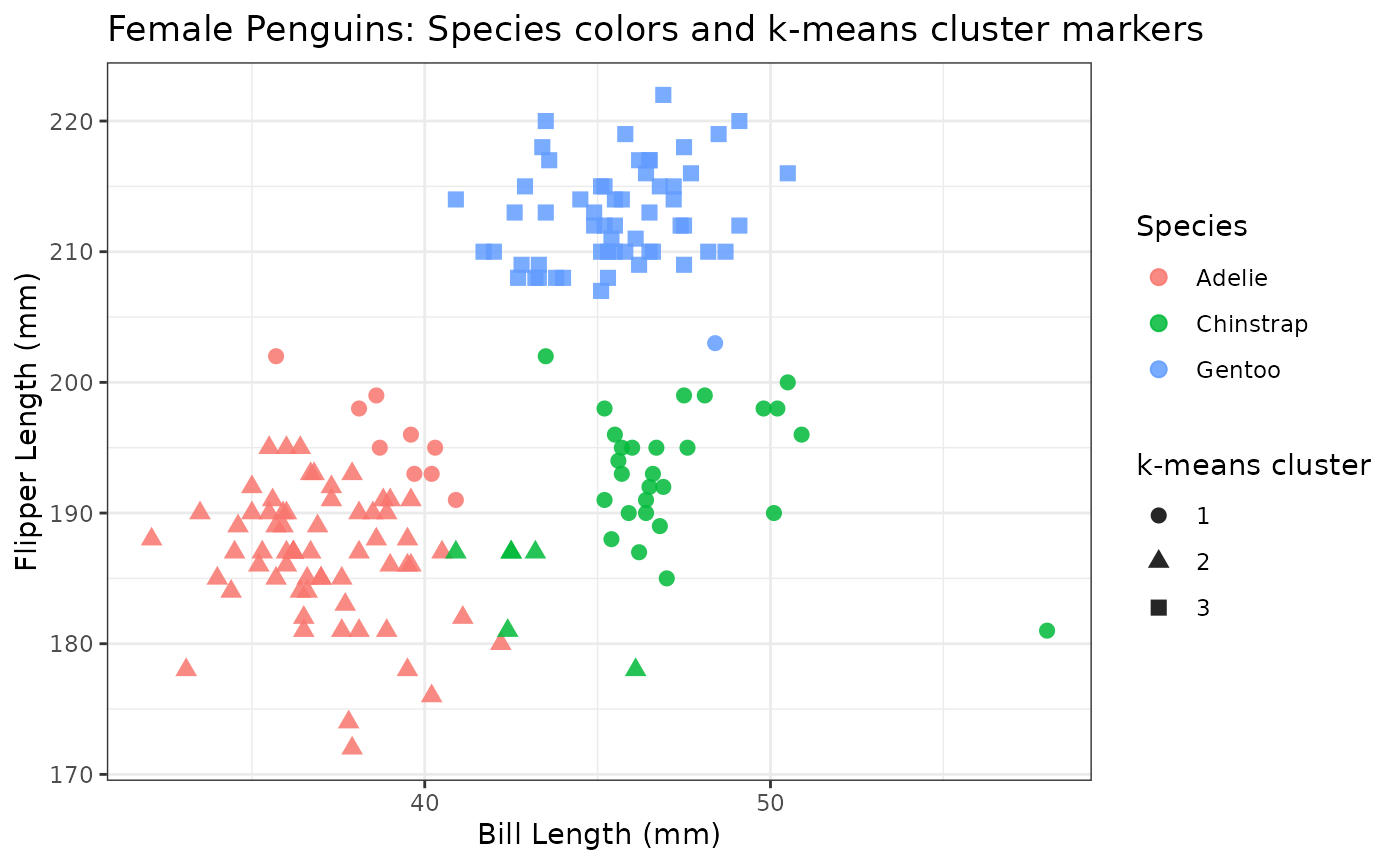
The same post-clustering inference analysis can also be performed using the k-means clustering algorithm. First, we classify the data into 3 groups with k-means. The resulting partition is shown below.

Performing k-means on the penguins data

# Perform k-means clustering
km_result <- kmeans(data_penguins[, c("bill_length_mm", "flipper_length_mm")], centers = 3)

# Extract cluster assignments
km_clusters <- km_result$cluster

# Scatter plot: color by species and use markers for k-means clusters
ggplot(data_penguins, aes(
  x = bill_length_mm,
  y = flipper_length_mm,
  color = species,
  shape = factor(km_clusters)
)) +
  geom_point(size = 2.5, alpha = 0.85) +
  theme_bw() +
  labs(
    title = "Female Penguins: Species colors and k-means cluster markers",
    x = "Bill Length (mm)",
    y = "Flipper Length (mm)",
    color = "Species",
    shape = "k-means cluster"
  )

Testing k-means clusters with `test.clusters.km()`

The test.clusters.km() function performs post-clustering inference for k-means clustering results. It has similar parameters to test.clusters.hc(), with the exception of the clustering algorithm specific parameters. Instead of specifying a linkage method, the user can specify:

📝 Note
For test.clusters.km(), the user can also provide an KmeansInference::kmeans_inference() object via the km_at_cl parameter. In this case, the function will not perform k-means again and will directly test the provided clustering result.

itermax: The maximum number of iterations allowed for the k-means algorithm to converge. The default is 10.
tol: The convergence threshold for the k-means algorithm. The default is 1e-6.

The remaining parameters are the same as in test.clusters.hc(). To use test.clusters.km(), simply replace the function name and specify the desired parameters. For example, to test the difference between clusters 1 and 2, we can run:

# Test the k-means clusters

km_test_12 <- PCIdep::test.clusters.km(X=X, Y=Y, NC = 3, clusters = c(1, 2)) # Using male penguins data to estimate covariance
#> U is not provided: observations are considered independent with unit variance.
#> Sigma not provided: plugging an over-estimate.
km_test_12$pvalue 
#> [1] 0.8053609

💡 Statistical power of test.clusters.km()
Post-clustering inference with k-means is generally less powerful than with HAC or other clustering algorithms. This is due to how the k-means p-value has been defined. The k-means p-value in PCIdep is an extension of that proposed by Chen and Witten, originally implemented for independent observations and features in the R package KMeansInference. The analytical tractability of this p-value requires conditioning on more information than in the HAC case, which comes at a price in conditional power. We refer the reader to Chen and Witten (2023) for a detailed discussion, or to the power analyses presented in the PCIdep paper.

Summary

In this vignette, we demonstrated how to perform post-clustering inference using the test.clusters.hc() and test.clusters.km() functions from the PCIdep package. For more details on the methods and assumptions underlying these functions, please refer to the package documentation and the PCIdep paper.