Inference after a custom clustering algorithm

Introduction

test.clusters.MC() allows to perform inference after any user-supplied clustering algorithm. This vignette walks through a complete example using HDBSCAN (Hierarchical Density-Based Spatial Clustering of Applications with Noise). For a user-friendly introduction to HDBSCAN, see the hdbscan package vignette or the python package documentation.

library(PCIdep)
library(dbscan)   
#> 
#> Attaching package: 'dbscan'
#> The following object is masked from 'package:stats':
#> 
#>     as.dendrogram
library(ggplot2)
library(MASS)

1. Simulate Data

In this example, we simulate a dataset with three “strands” of points drawn from three multivariate Gaussian distributions. This type of structure can be encountered in real-world data and can be challenging for some clustering algorithms to capture.

set.seed(42)

n <- 200   # Number of points per cluster
Sigma <- matrix(c(2.5, -0.99, -0.99, 0.45), nrow = 2) # Covariance matrix

# Three Gaussian strands
g1 <- MASS::mvrnorm(n = n, mu = c(-5, 0), Sigma = Sigma)
g2 <- MASS::mvrnorm(n = n, mu = c(0, 0), Sigma = Sigma)
g3 <- MASS::mvrnorm(n = n, mu = c(2, -3), Sigma = Sigma)

X <- as.matrix(rbind(g1, g2, g3))
colnames(X) <- c("x", "y")
df <- as.data.frame(X)

# Plot raw simulated data
ggplot(df, aes(x = x, y = y)) +
  geom_point(alpha = 0.6, size = 1.8) +
  ggtitle("Simulated data") +
  theme_bw()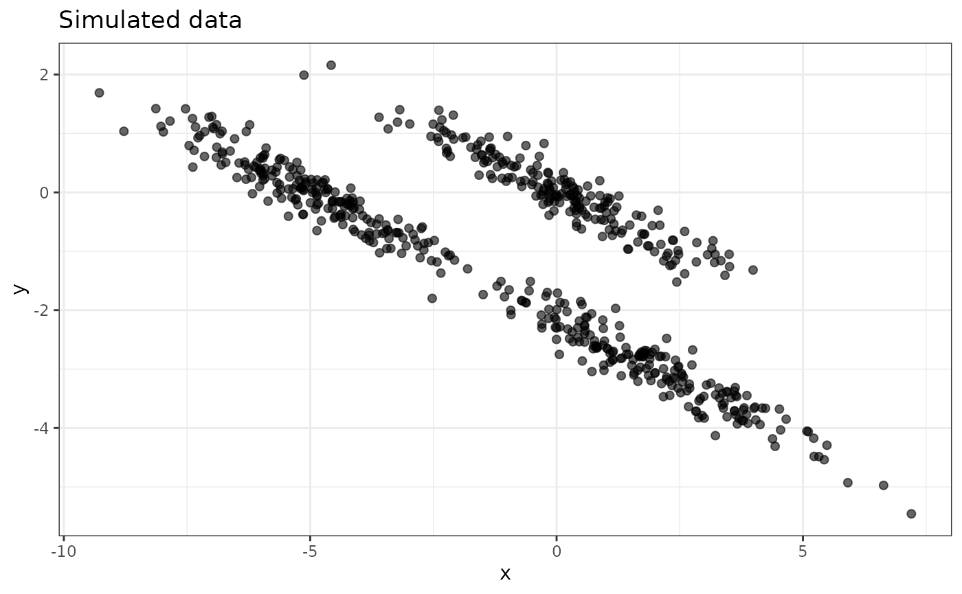

2. Construct the Cluster Function

We are interested in clustering the data using HDBSCAN and then testing for differences in cluster means between two of the identified clusters. To do so, we need to construct a function wrapping the HDBSCAN algorithm that can be passed to test.clusters.MC(). The wrapper must take as input the data matrix and return a vector of cluster labels. In the case where the custom clustering algorithm requires the number of clusters to be specified, the wrapper should also take an argument NC and pass it to the clustering function. In the case of HDBSCAN, the number of clusters is determined automatically, so we do not need to use NC in our wrapper. Any other hyperparameters of the clustering algorithm should be exposed as arguments of the wrapper function so that they can be tuned easily. In the case of HDBSCAN, a key hyperparameter is minPts (the minimum cluster size), which we include in our wrapper.

test.clusters.MC() requires a cl_fun argument that follows this interface:

cl_fun(X, NC, ...) → integer vector of length nrow(X)

X is the data matrix passed to test.clusters.MC().

NC is the number of clusters (if required by the clustering algorithm). If chosen automatically, the NC argument can be omitted.

The return value must be an integer (or integer-coercible) vector where each element is the cluster label for the corresponding observation.

hdbscan_fun <- function(X, minPts = 10) {
  res    <- dbscan::hdbscan(X, minPts = minPts) # minPts controls the minimum cluster size in HDBSCAN.
  labels <- as.integer(res$cluster)
  return(labels)
}

Note: If the clustering algorithm requires the number of clusters NC explicitly, it must be passed to cl_fun. For example, a kmeans wrapper for test.clusters.MC() can be written as:

kmeans_fun <- function(X, NC, nstart = 10) {
  fit <- stats::kmeans(X, centers = NC, nstart = nstart)
  as.integer(fit$cluster)
}

Let us verify that the hdbscan_fun works on our simulated data:

labels_hdbscan <- hdbscan_fun(X, minPts = 10)
df$hdbscan_cluster <- factor(labels_hdbscan)

ggplot(df, aes(x = x, y = y, colour = hdbscan_cluster)) +
  geom_point(alpha = 0.7, size = 1.8) +
  scale_colour_brewer(palette = "Set1", name = "Cluster\n(0 = noise)") +
  ggtitle("HDBSCAN cluster labels") +
  theme_bw()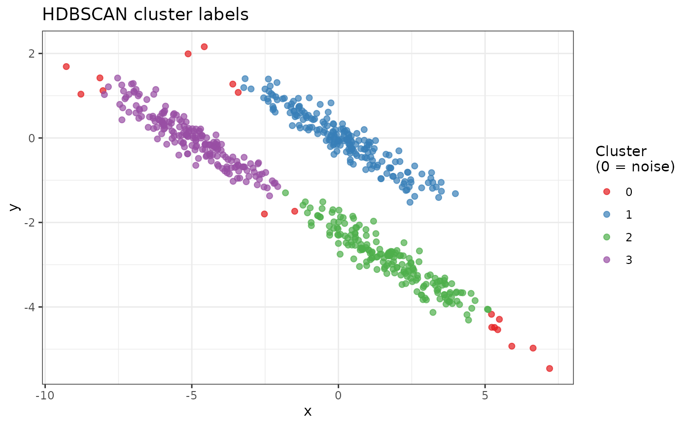

3. Run `test.clusters.MC()`

test.clusters.MC() computes a Monte Carlo based p-value to assess whether the means of a pair of clusters found by the algorithm are significantly different. The function takes the same list of parameters as the test.clusters.hc() and test.clusters.km() functions, with the exception of the cl_fun and ndraws arguments:

Key arguments:

Argument	Description
`cl_fun`	The wrapper function built in the previous section.
`ndraws`	Number of Monte Carlo iterations (larger → more precise p-values).

⚠ Covariance estimation
The same considerations as in the HAC and k-means cases apply. Here, we use sample splitting to generate an i.i.d. copy of the data for covariance estimation.

💡 Use of parallel computation
The p-value is computed via Monte Carlo simulation: the clustering algorithm is run ndraws times on perturbed data, and the results are aggregated to approximate the null distribution of the test statistic. Since each Monte Carlo draw is independent, the computation can be parallelized straightforwardly using the future package. Simply call plan() before running the test and choose the number of workers according to your machine’s available cores.

set.seed(123)

library(future) 
plan(multisession, workers = 5) # Set parallelization plan (adjust workers according to your machine)
#> Warning in checkNumberOfLocalWorkers(workers): Careful, you are setting up 5
#> localhost parallel workers with only 4 CPU cores available for this R process
#> (per 'system'), which could result in a 125% load. The soft limit is set to
#> 100%. Overusing the CPUs has negative impact on the current R process, but also
#> on all other processes of yours and others running on the same machine. See
#> help("parallelly.maxWorkers.localhost", package = "parallelly") for further
#> explanations and how to override the soft limit that triggered this warning

# Compare clusters 1 and 2
res_12 <- test.clusters.MC(X, clusters = c(1, 2), cl_fun = hdbscan_fun, NC = NULL, cl = NULL, ndraws = 500, sample_split = TRUE)
#> Warning in test.clusters.MC(X, clusters = c(1, 2), cl_fun = hdbscan_fun, : The
#> sample used for clustering is a subsample of the one introduced as input (as
#> sample_split is TRUE). Consider setting return_X_clus to TRUE for further
#> analysis of the retrieved clusters.
#> U is not provided: observations are considered independent with unit variance.
#> Sigma not provided: plugging an over-estimate.
res_12$pvalue
#> [1] 8.828849e-06

# Compare clusters 2 and 3
res_23 <- test.clusters.MC(X, clusters = c(2, 3), cl_fun = hdbscan_fun, NC = NULL, cl = NULL, ndraws = 500, sample_split = TRUE)
#> Warning in test.clusters.MC(X, clusters = c(2, 3), cl_fun = hdbscan_fun, : The
#> sample used for clustering is a subsample of the one introduced as input (as
#> sample_split is TRUE). Consider setting return_X_clus to TRUE for further
#> analysis of the retrieved clusters.
#> U is not provided: observations are considered independent with unit variance.
#> Sigma not provided: plugging an over-estimate.
res_23$pvalue
#> [1] 0.001599352

# Compare clusters 1 and 3
res_13 <- test.clusters.MC(X, clusters = c(1, 3), cl_fun = hdbscan_fun, NC = NULL, cl = NULL, ndraws = 500, sample_split = TRUE)
#> Warning in test.clusters.MC(X, clusters = c(1, 3), cl_fun = hdbscan_fun, : The
#> sample used for clustering is a subsample of the one introduced as input (as
#> sample_split is TRUE). Consider setting return_X_clus to TRUE for further
#> analysis of the retrieved clusters.
#> U is not provided: observations are considered independent with unit variance.
#> Sigma not provided: plugging an over-estimate.
res_13$pvalue
#> [1] 1.677807e-05

future::plan(future::sequential) # Reset to sequential plan to avoid leaking workers

The reported p-values indicate that the clusters are significantly different.

Conclusion

This vignette demonstrated how to use test.clusters.MC() for inference after custom clustering algorithms. The key steps are:

Define a wrapper function that implements your clustering algorithm and returns integer cluster labels.
Run test.clusters.MC() with your wrapper function to obtain Monte Carlo-based p-values for pairwise cluster comparisons.
Parallelize computation using the future package for faster inference on large datasets.

Introduction

1. Simulate Data

2. Construct the Cluster Function

3. Run test.clusters.MC()

Conclusion

3. Run `test.clusters.MC()`