
Why post-clustering inference?
Clustering is one of the most common exploratory tools in statistics, biology, and data science. In a typical workflow, we observe a data matrix \mathbf{X} \in \mathbb{R}^{n \times p}, where the rows are observations and the columns are features. For example, the rows may be protein conformations, patients or cells, while the columns may be molecular distances, gene expression measurements, or other quantitative descriptors. A clustering algorithm is then applied to the data in order to identify groups of similar observations. In many applications, these groups are interpreted as reflecting underlying biological, genetic, or functional structure in the data. However, clustering is fundamentally an exploratory task, and interpreting its output is often much more difficult than obtaining the clustering itself. In practice, clustering raises several important statistical and interpretability questions:
- What exactly is a cluster?
- How stable are the discovered groups?
- Do the detected clusters correspond to biologically meaningful differences?
- Can apparent clusters arise purely from noise?
Answering these questions rigorously requires statistical tools capable of quantifying uncertainty after the clustering step has already been performed. In other words, we need to answer the question:
Are the clusters really different?
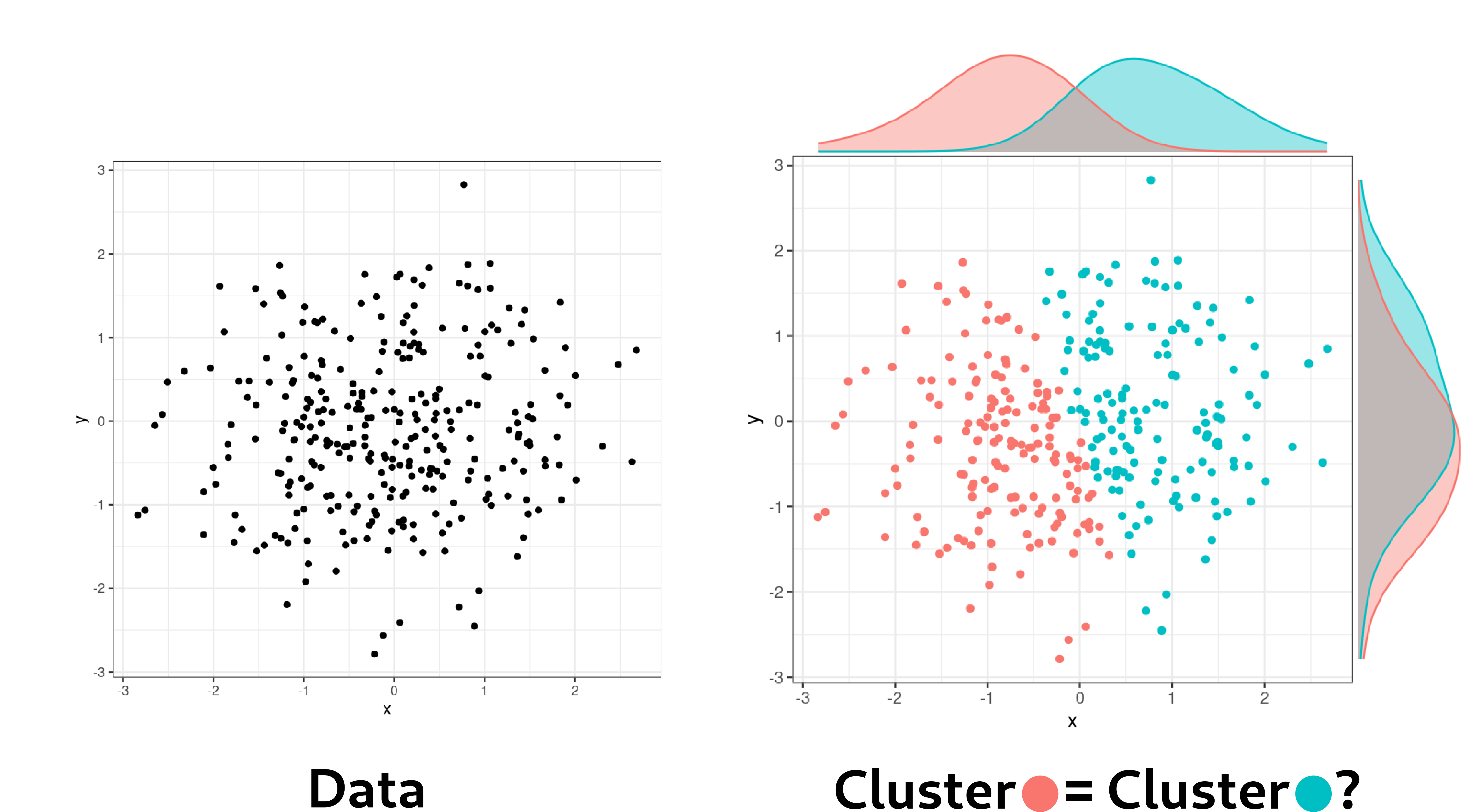
At first sight, this looks like a standard two-sample testing problem. However, there is a crucial complication: the clusters (and therefore the hypothesis to test) have been selected from the data.
⚠ The double-dipping
problem
The problem is often called double
dipping: the same data are used twice, first to discover the
clusters and then to test whether those clusters differ. If we ignore
this selection step and apply a classical test as if the clusters had
been fixed in advance, the resulting p-values lose the type I error control. This
happens because clustering algorithms are designed to find groups that
look different. If we then test the difference between those same groups
without accounting for the fact that they were selected to be different,
we underestimate the amount of randomness involved.
A small simulation: why naive inference fails
To illustrate the double-dipping issue in a simple setting, we simulate data with no true cluster structure: each observation is generated from the same Gaussian distribution. We then apply k-means clustering, randomly pick two of the resulting clusters, and perform a classical test comparing their empirical means. Repeating this many times shows what happens when the clustering step is ignored: under the null hypothesis the resulting p-values are no longer approximately uniform, revealing the inflation of false positives caused by naive post-clustering inference.
set.seed(1)

simulate_naive_pvalue <- function(n = 60, p = 5, k = 3) {

  X <- matrix(rnorm(n * p), nrow = n, ncol = p)
  cl <- kmeans(X, centers = k, nstart = 10)$cluster

  groups <- split(seq_len(n), cl)
  pair <- sample(seq_along(groups), 2)

  g1 <- groups[[pair[1]]]
  g2 <- groups[[pair[2]]]

  x1 <- X[g1, , drop = FALSE]
  x2 <- X[g2, , drop = FALSE]

  diff <- colMeans(x1) - colMeans(x2)
  s2 <- apply(X, 2, var)

  stat <- sum(
    diff^2 /
    (s2 * (1 / length(g1) + 1 / length(g2)))
  )

  pchisq(stat, df = p, lower.tail = FALSE)

}

B <- 500
p_naive <- replicate(B, simulate_naive_pvalue())

alpha <- c(0.01, 0.05, 0.10)
fp_rate <- sapply(alpha, function(a) mean(p_naive < a))

knitr::kable(
  data.frame(
    `Significance level` = paste0(alpha * 100, "%"),
    `Expected false positive rate` = paste0(alpha * 100, "%"),
    `Observed false positive rate` = paste0(round(fp_rate * 100, 1), "%"),
    check.names = FALSE
  ),
  align = "ccc",
  caption = "Proportion of rejections under the null hypothesis using naive inference after k-means clustering (500 simulations). Without accounting for the clustering step, the false positive rate is severely inflated above the nominal level."
)| Significance level | Expected false positive rate | Observed false positive rate |
|---|---|---|
| 1% | 1% | 100% |
| 5% | 5% | 100% |
| 10% | 10% | 100% |
Addressing double-dipping
Selective inference is the statistical theory that aims, among other goals, to provide principled strategies to avoid double-dipping when the model, hypothesis, or question is chosen adaptively from data. In this data-driven setting, the literature proposes several families of approaches, including (but not limited to): simultaneous inference, universal inference, sample splitting, data fission/thinning, and conditional inference. Up-to-date, only conditional-based approaches have been shown efficient in the context of inference after clustering, starting with the seminal work of Gao et al. (JASA, 2022).
💡 Suitability of data
fission/thinning for post-clustering inference
The
suitability of techniques like data fission/thinning (Leiner et
al., 2023, Neufeld et
al., 2025) still remains an open question in the context of
inference after clustering. Despite notable recent advances in
parameter estimation, robust estimation in the context of clustering
remains unclear, as discussed by Hivert et
al. (2026).
Selective type I error: the conditional inference approach
Post-clustering inference aims to control the probability of false rejection conditional on the clustering event. This is referred to as selective type I error control. More formally, if \mathcal{C}(\mathbf{X}) denotes the clustering partition obtained from the data and C_1, C_2 are two clusters found by the algorithm, the selective type I error is controlled at level \alpha if
\mathbb{P}_{H_0^{\{C_1,C_2\}}} \left( \text{reject } H_0^{\{C_1,C_2\}} \mid C_1,C_2 \in \mathcal{C}(\mathbf{X}) \right) \leq \alpha,
where H_0^{\{C_1,C_2\}} is the null hypothesis of equality of clusters that needs to be specified for a given data model.
The PCIdep approach
The statistical model
The PCIdep package is designed for post-clustering
inference under a matrix
normal model with possible dependence between observations and/or
features:
\mathbf{X} \sim \mathcal{MN}_{n \times p}(\boldsymbol{\mu}, \mathbf{U}, \boldsymbol{\Sigma}).
Here:
- \boldsymbol{\mu} \in \mathbb{R}^{n \times p} is the mean matrix;
- \mathbf{U} \in \mathbb{R}^{n \times n} describes dependence between observations;
- \boldsymbol{\Sigma} \in \mathbb{R}^{p \times p} describes dependence between features.
This means that:
- Every row X_i of \mathbf{X} is distributed as \mathcal{N}_p(\mu_i, U_{ii}\boldsymbol{\Sigma}),
- Every column X^j of \mathbf{X} is distributed as \mathcal{N}_n(\mu^j, \Sigma_{jj}\mathbf{U}),
- The covariance between two entries X_{ij} and X_{i'j'} is given by \mathrm{Cov}(X_{ij}, X_{i'j'}) = U_{ii'} \Sigma_{jj'},
or, equivalently,
\mathrm{vec}(\mathbf{X}) \sim \mathcal{N}_{np}\left(\mathrm{vec}(\boldsymbol{\mu}), \boldsymbol{\Sigma} \otimes \mathbf{U}\right).
In this setting, independent observations correspond to \mathbf{U} = \mathbf{I}_n, while independent features correspond to \boldsymbol{\Sigma} = \sigma^2\mathbf{I}_p.
The null hypothesis
In this model, the equality of clusters C_1 and C_2 is expressed as the equality of cluster means, defined as \bar{\mu}_{C} = \frac{1}{|C|} \sum_{i \in C} \mu_i for any cluster C. This means that the null hypothesis is written as:
H_0^{\{C_1,C_2\}}: \bar{\mu}_{C_1} = \bar{\mu}_{C_2}.
Model assumptions to compute a p-value
\mathbf{U} must be known and compound symmetric
In the PCIdep paper, we show that a p-value for H_0^{\{C_1,C_2\}} can be computed in closed form, provided that the dependence structure between observations \mathbf{U} is known and belongs to the class of compound symmetry matrices.
⚠ \mathbf{U} must be compound symmetric
The class \mathcal{CS}(n) of compound symmetry matrices of size n is defined as:
\mathcal{CS}(n) = \left\{ (a-b)\mathbf{I}_n + b\mathbf{1}_{n\times n} : a \ge 0, -\frac{a}{n-1} < b < a \right\}.
where \mathbf{1}_{n\times n} is the n \times n matrix of ones. In the PCIdep paper, we show that the testing procedure is robust to deviations from \mathcal{CS}(n), so that the method can be applied in practice if the known matrix \mathbf{U} does not present substantial deviations from the compound symmetry class (e.g. for autoregressive processes).
Note that the case of independent observations is trivially included in this setting, since the identity matrix belongs to \mathcal{CS}(n).
The closed form of the p-value when \mathbf{U} \in \mathcal{CS}(n) is detailed in Section 2 of the PCIdep paper.
\boldsymbol{\Sigma} can be unknown and arbitrary
One of the main contributions of the PCIdep approach is
that the dependence structure between features \boldsymbol{\Sigma} can be unknown and
estimated in practice, while respecting the validity of the resulting
p-value.
💡 In practice
The
functions in PCIdep automatically estimate \boldsymbol{\Sigma}. As statistical
guarantees are respected asymptotically, the sample size n should be sufficiently large for the
resulting p-values to be valid.
Technical details on the estimation of \boldsymbol{\Sigma} and the resulting asymptotic validity of the p-values are provided in Section 3 of the PCIdep paper.
PCIdep in practice
This vignette introduced the statistical motivation of
post-clustering inference, the matrix normal model used in
PCIdep, and the selective framework behind valid p-values after clustering. To see how to
compute these p-values and use
PCIdep in practice:
- For hierarchical agglomerative clustering (HAC) and k-means, see the HAC and k-means vignette.
- For user-defined or custom clustering procedures, see the custom clustering vignette.